Programming Languages
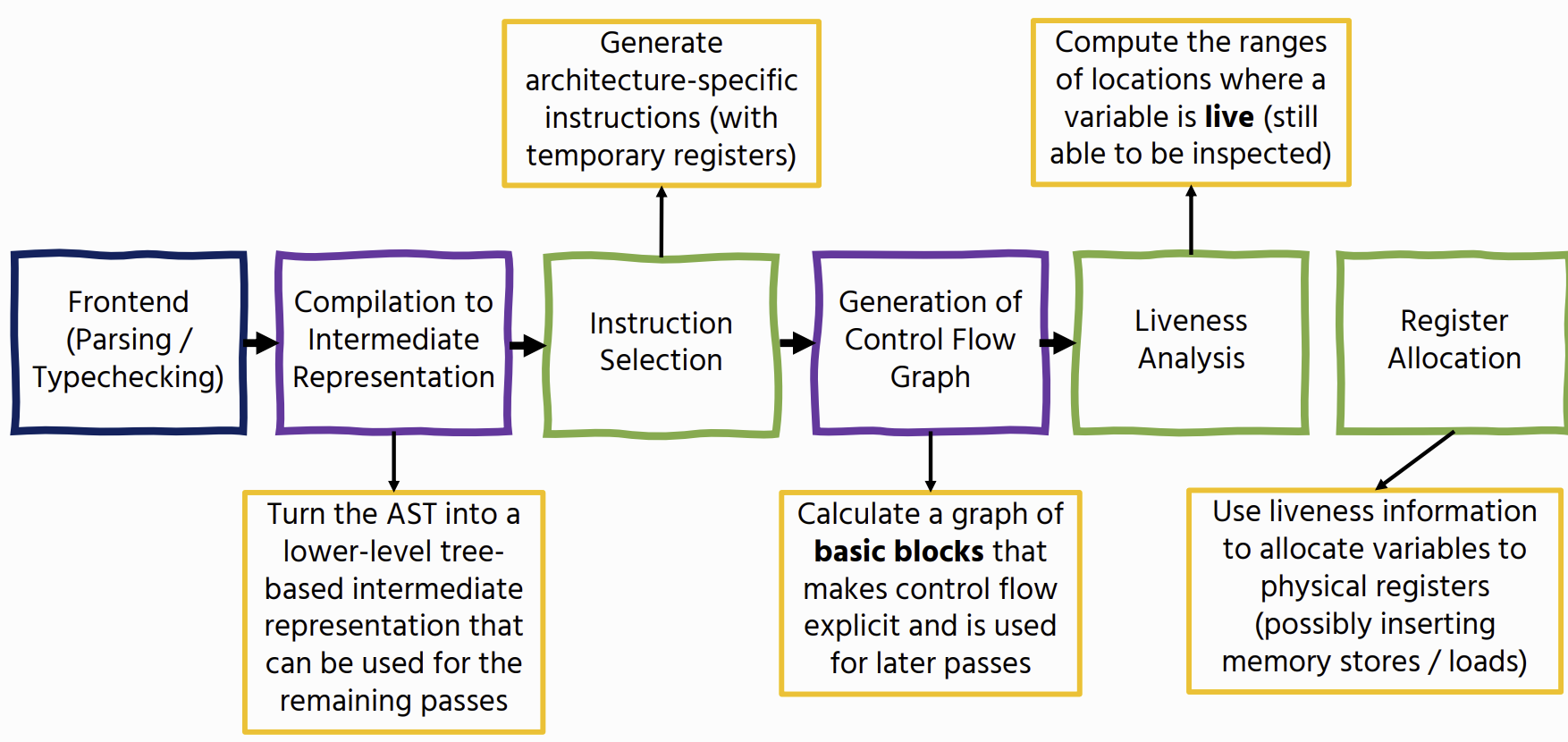
Pipeline
parsing : transform source code (strings) into a structured representation → Type checking : Check that source code does not have type errors (for typed languages) → Desugaring : translate complicated constructs into smaller ones (dont have to duplicate logic) → IR Conversion : translate into intermediate representation → Optimisation → Compilation/Interpretation: Either interpret the code, emit lower-level code
Also we need a Runtime e.g. Garbage collection
Components
Syntax
constructs of language, how does it look?
Typing Rules (if language is typed)
what programs are sensible? can we rule out errors?
Semantics
what does a program mean? what should it do when it is run?
Programming Paradigms
style of programming that dictates the principles, techniques, and methods used to solve problems in that language use the right tool for the job
Expressions vs Statements
Expressions - A term in the language that eventually reduces to a value (can be contained within a Statement) Statement - An instruction / computation step, does not return anything
Imperative Programming Language
Program Counter + Call stack + State i.e. c, Python, JavaScript record our current position in the program, Statements can alter that position Variable assignments alter some store
Imperative paradigm closer to the underlying hardware as it is built around mutability
Functional Programming Language
everything is an expression first-class functions: can create, apply, and pass functions just like any other expression Evaluation is reduction of a complex expression to a value
Object-Oriented Programming Language
object: consists of some state (fields), and some functions that operate on the state (methods) encapsulation: don’t expose internal state unnecessarily inheritance: ability to extend previously-defined objects to make new ones
Syntax
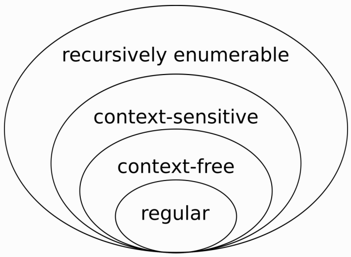 | Regular expressions are regular languages Context-free languages can be recognised by a push-down automaton Context-sensitive languages and recursively enumerable languages require more interesting recognisers |
Grammar
set of formal rules specifying how to construct a sentence in a language. it consists of:
- A set of terminal symbols: symbols that occur in a sentence
- the keywords that end
- A set of nonterminal symbols, which each ‘stand for’ part of a phrase
- the expression keyword that would not end
- A distinguished sentence symbol that stands for a complete sentence
- what do you want to parse, where you start from
- A set of production rules that show how phrases can be made up from terminals and sub-phrases
- the symbol that make up phrases
Backus-Naur Form (BNF) - Concrete Syntax
BNF grammar consists of a series of productions takes the form S ::= a|b|c
expr ::= prim | expr op prim
op ::=  '+'  |  '-'  |  '*'  |  '/'
prim ::= int | '(' expr ')'
int ::= digit
digit ::= '1' | '2' | '3' | '4' | '5' | '6' | '7' | '8' | '9' | '0'
Extended BNF (EBNF) allows us to use regular expressions i.e. if digit+ (one or more digits)
Parse Tree
a parse tree corresponds a string to a grammar
| ![[parse tree.png|]] | Each terminal node is labelled by a terminal symbol (here, digits and operators) Each nonterminal node is labelled by a nonterminal symbol of G and can have children nodes X, Y, Z only if G has a production rule N ::= … | X Y Z | … |
Abstract Syntax
allows us to abstract away irrelevant syntactic noise (focus on the important parts)
Integers n
Operators ⊙ ::= + | - | * | /
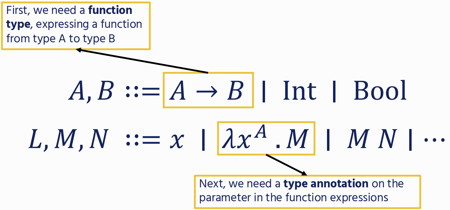
Terms L, M, N ::= n | L ⊙ M
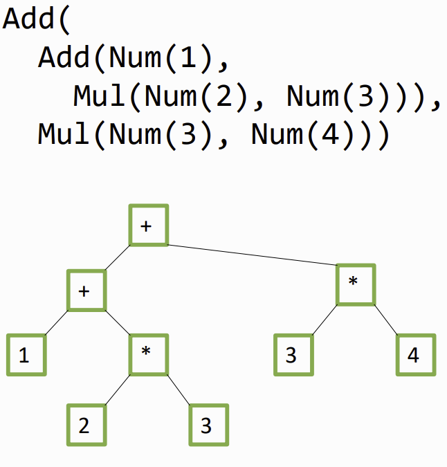
Abstract Syntax Tree
a way to represent a parsed program the steps to parse text into an AST is:
- Tokenise text into chunks using regular expressions (lexing)
- Match token streams and convert these into AST nodes (parsing)
on the example : (1 + 2 * 3) + (3 * 4)
Evaluation
Compiler
compiler translates code into lower-level languages, such that eventually they can be executed on hardware often, compiled code needs to be supported by a runtime system
Interpreter
a program that accepts a program written in a given programming language, and executes it directly (no sperate executable) interpreters are easier to write but slower than compiled code
Virtual Machines
evaluates instructions (usually encoded in some sort of bytecode) by an interpreter
- platform independance: Can run compiled code on multiple platforms
- Common backend: multiple (quite different) languages can target the same backend
Just-in-time (JIT) Compilers
a middleground between compilers and interpreters, where code is compiled to native code at run-time JIT compilers operate selectively: they profile code and compile frequently called code
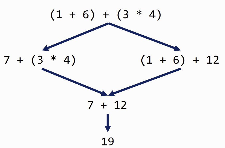
Operational Semantic
Big-step: Closer to how we write interpreters, but cannot reason easily about nonterminating expressions Small-step: More fine-grained reasoning power, but (usually) further away from how we would implement a language
Determinism & Church-Rosser Theorem
no matter which path you take in computation, the answer is always the same (no side-effects)
Semantic Approaches
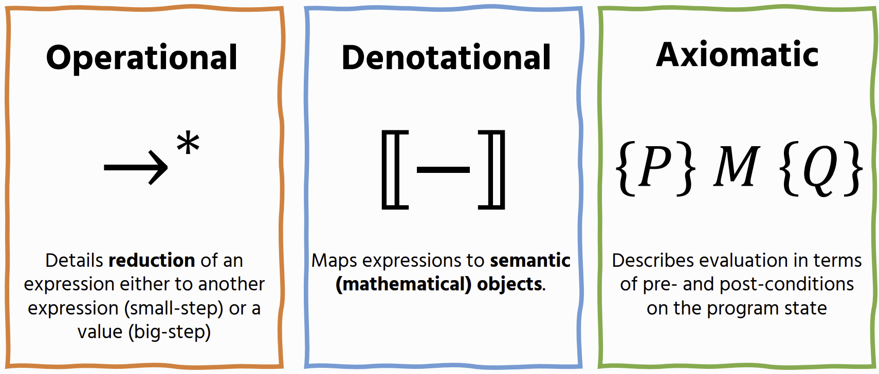
Textual Descriptions
plain English on how expressions work but can be very ambigus
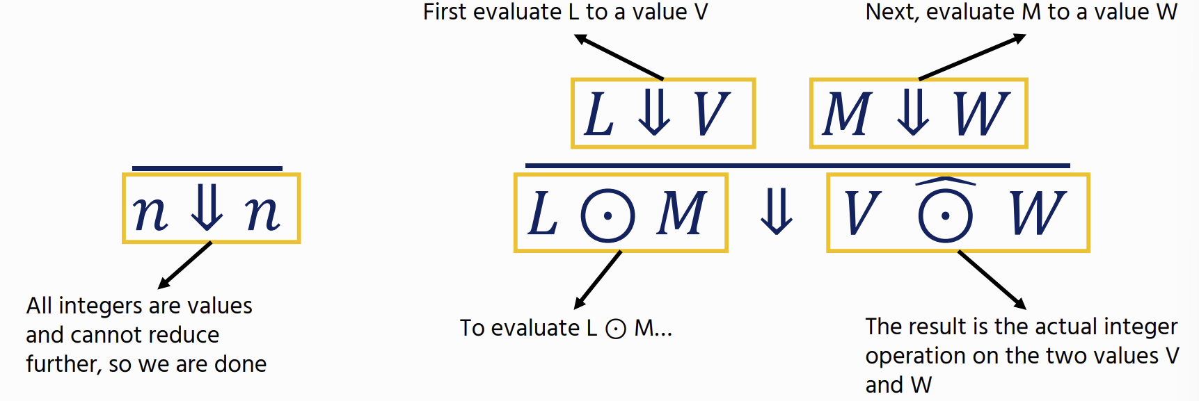
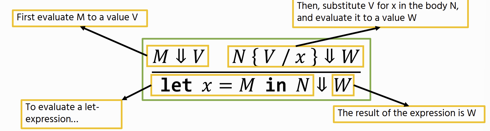
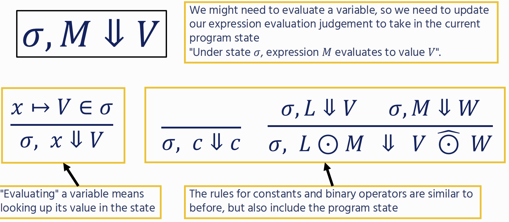
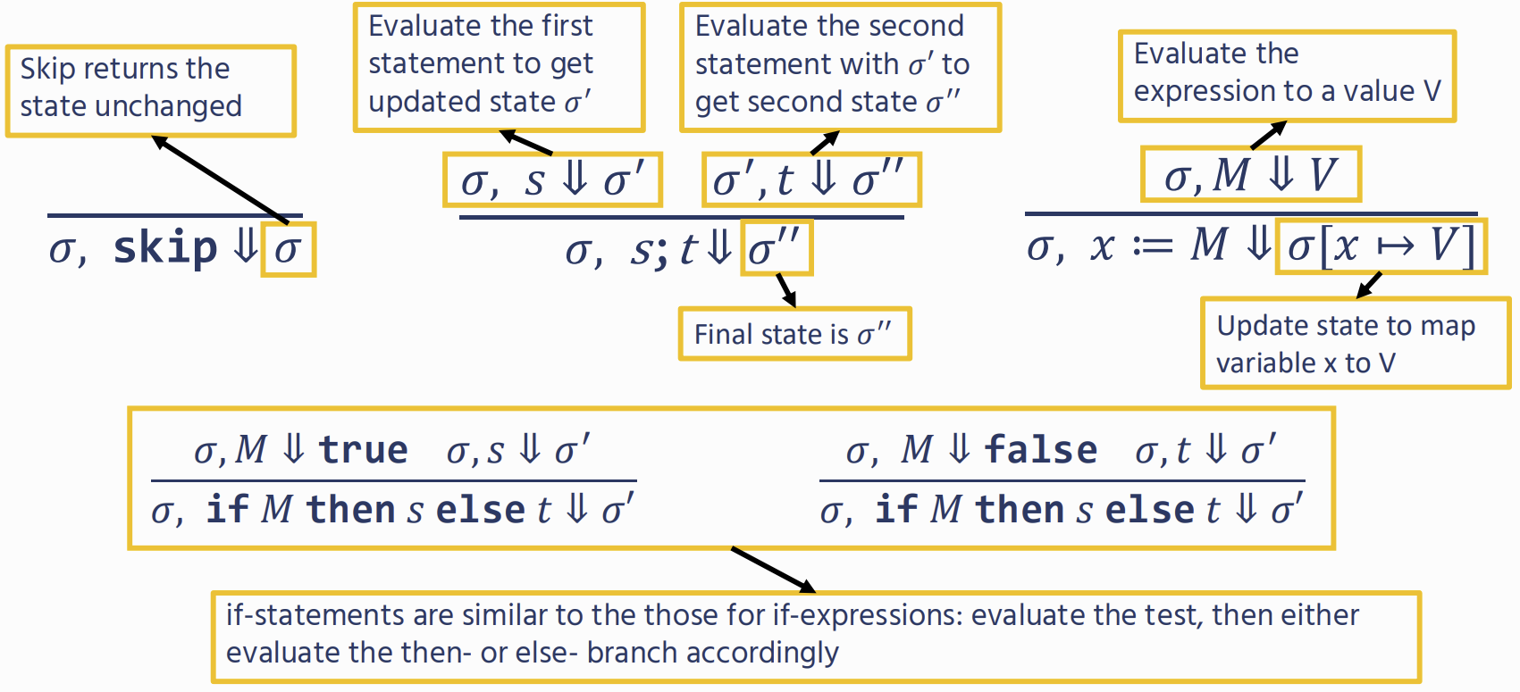
Big-Step Operational Semantics
Theorem: If ⋅⊢ M ∶ A then there exists some V such that M ⇓ V and ⋅ ⊢ V: A.
M ⇓ V : shows how an expression M evaluates to a value V. (aka a judgement)
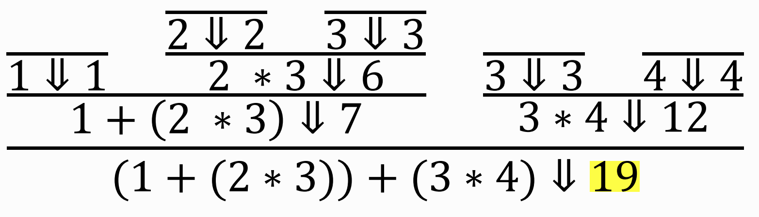
derivation tree for L_arith
Small-Step Operational Semantics
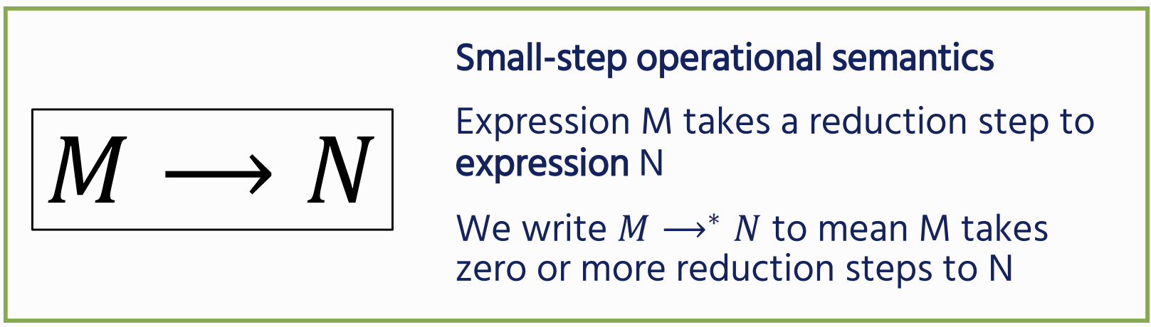 The idea is that we repeatedly apply the congruence rules (like evaluating the test subexpression) until we can evaluate the actual reduction step
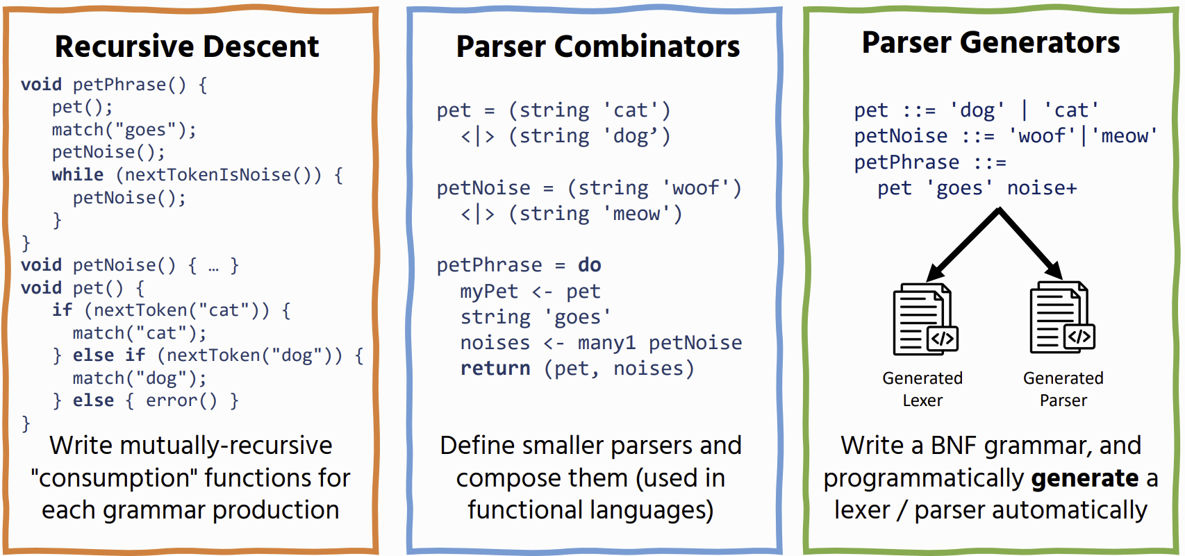
Parsing
Parsers take unstructured text and turn it into a structured representation (parse tree) based on the rules of a grammar
Lexing
process of turning unstructured text into a token stream, so that it can be more easily consumed by a parser
1 + (2 * 3) - 1 → INT(1), LPAREN, INT(2), STAR, INT(3), RPAREN, MINUS, INT(1)
Parsing
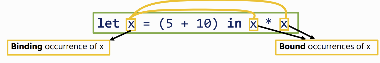
Bindings
Let Bindings
Variables
Free Variables
bound variables are considered free variables
fv(x) = {x} : x on its own is a free variable
fv(n) = ∅ : Integer literals don’t contain variables
fv(M ⊙ N) = fv(M) ∪ fv(N) : The free variables of a binary operator are the union of the free variables of its operands
fv(let x = M in N) = fv(M) ∪ (fv(N) \ {x}) : Any free occurrence of x would be bound by the let, so we need to remove it from the set of N’s free variables
Name shadowing
let x = 5 in
let x = 10 in
x + x
the x on line3 are all bound by the second let, therefore no-free variables The first let-binder is redundant, and has been shadowed by a more recent binder
Substitution
M {V / x} : Replace all free occurrences of x in term M with value V
Let Variable Operational Semantics
 There is no rule for trying to evaluate a free variable is an error
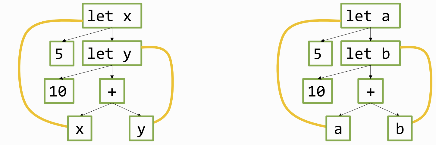
α-equivalence
two expressions are the same, as long as their binding structure is the same. to do this we can only rename bound variables. we Cannot:
- change names of free variables
- change the binding structure
- change the syntax
- change order of variables
best way to calculate is a binding diagram:
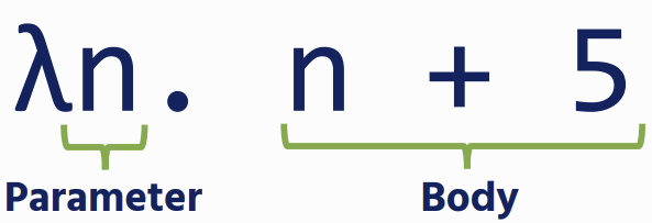
Functions
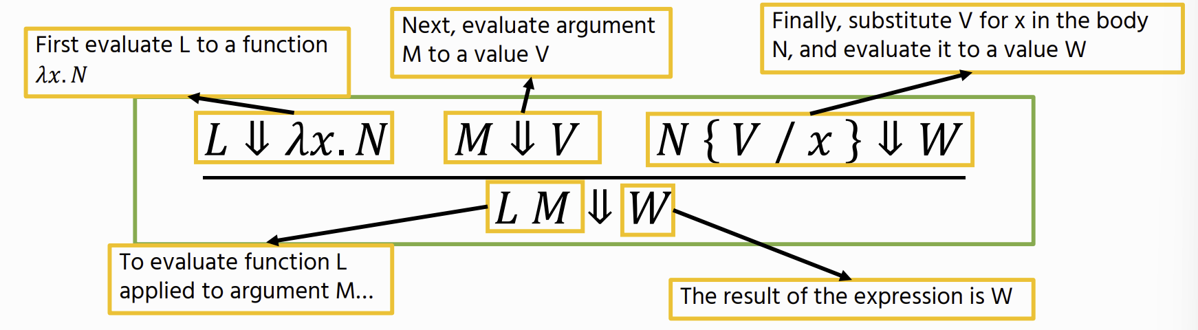
Anonymous (lambda) functions
 then apply a function, meaning we replace the free occurrences of the parameter with an argument before evaluating

Multi argument functions
ambda expressions only have a single parameter, but we can define functions with multiple parameters by nesting multiple functions
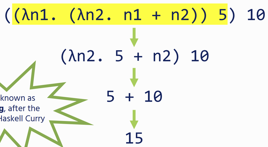 This is Known as Currying
lambda Operational Semantics
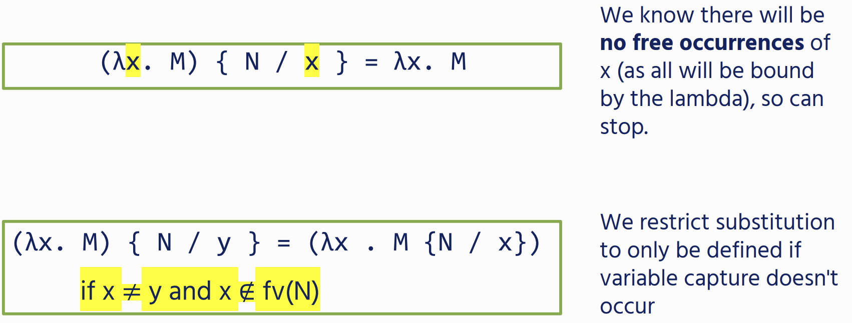
Capture-Avoiding Substitution
Variable Capture
where a free variable becomes bound after substitution. This can change the meaning of the expression.
To Avoid this we can use α-equivalence to pick fresh var names, whenever we need to substitute under a binder
 if a substitution causes variable capture, you can rename the variable - Barendregt’s Convention
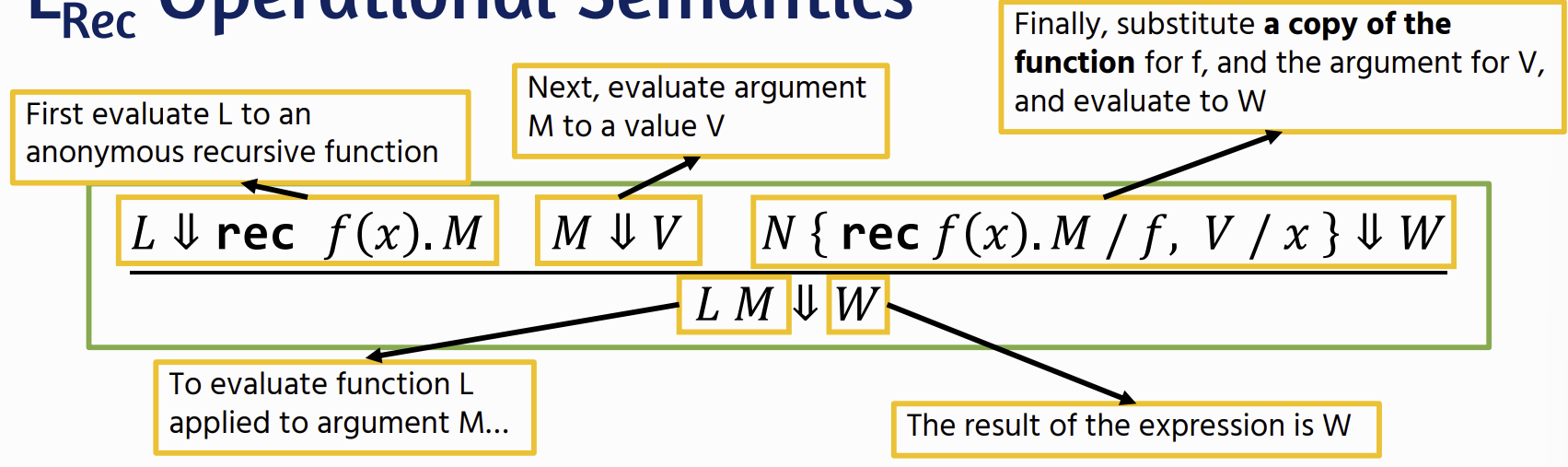
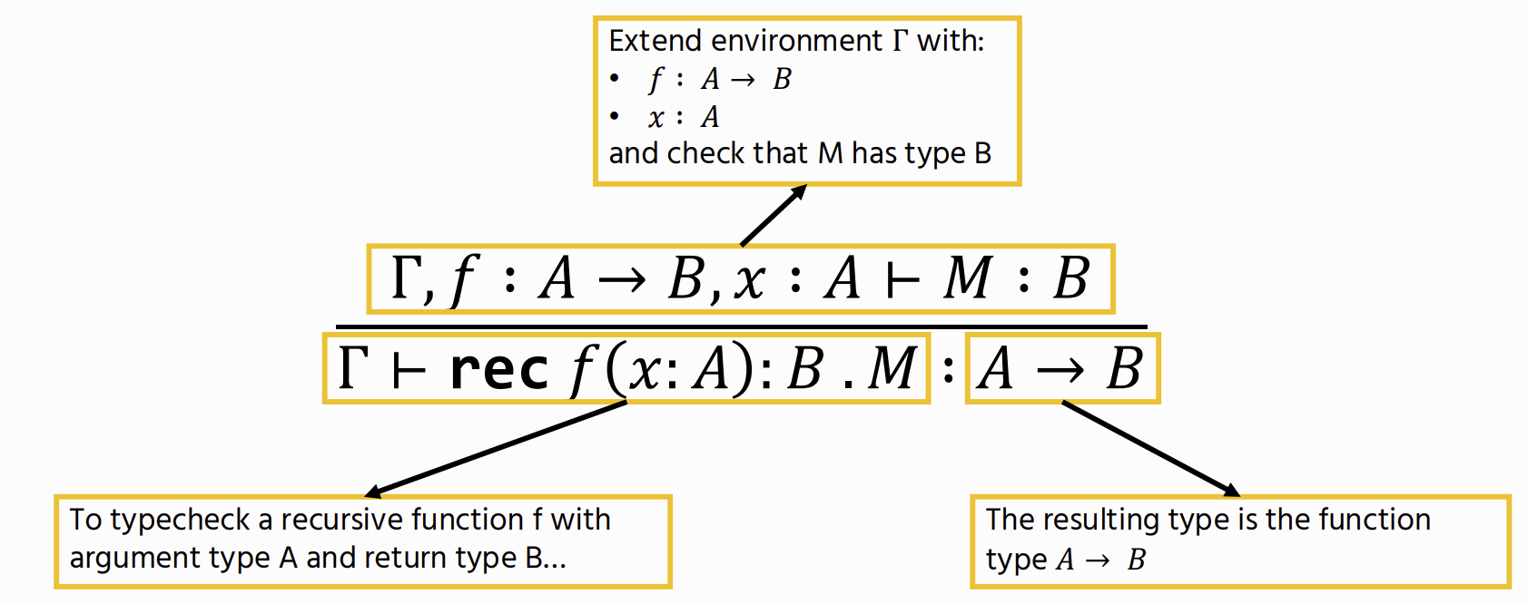
Recursion
Recursion Operational Semantics
Types
⊢ M : A “Term M has type A”
Typing Rules
Addition
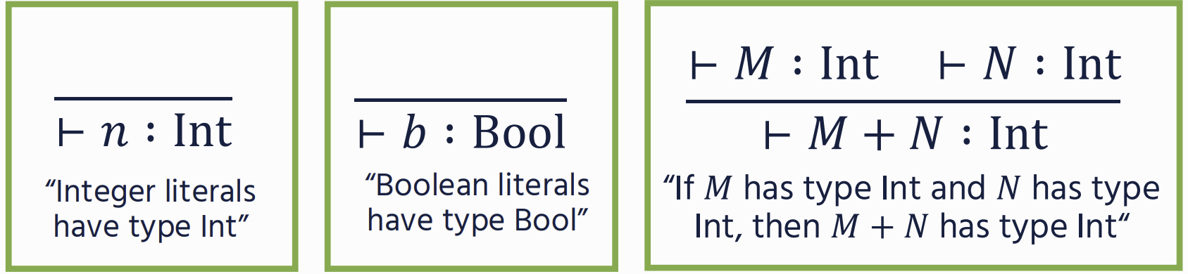
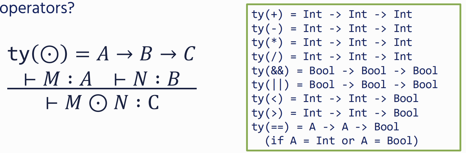
Binary operators
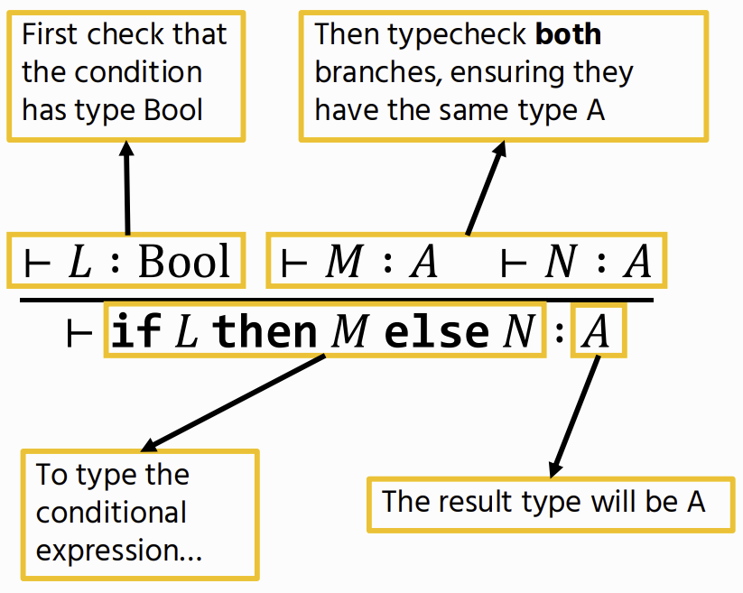
Conditionals
Type Environment
used for Functions
Γ ::= ⋅ ∣ Γ, x : A - a mapping from variables to types
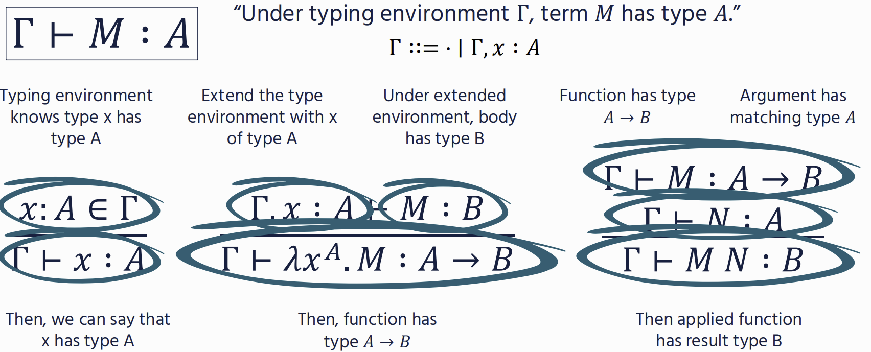
Functions
Recursive Function
Type Checking
Static - all typechecking happens before a program is run
- Lower memory cost / runtime Dynamic - tag values with their types, and perform typechecking dynamically to avoid crashes
- flexible, allowing branching control now where branches have different types.
Data Types
Encodability
- Records can be encoded using products
- Variants can be encoded using sums
- Booleans can be encoded using sums and the unit type local encodings: we can replace one construct with another as if it were a macro. global encodings: require us to rewrite a program (e.g. by adding a parameter to every function)
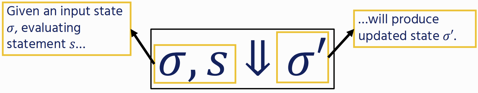
Imperative Programming
we’re not trying to produce a value, but instead modify the program state
Type Soundness
If a program is well typed, then it is either already a value, or it can take a step while staying well typed
If ⋅ ⊢ M ∶ A, then either M is a value A, or there exists some N such that M ⟶ N and ⋅ ⊢ N ∶ A.
Preservation
Reduction doesn’t change the result type or introduce type errors
If Γ ⊢ M : A and M −→ N, then Γ ⊢ N : A.
Progress
Well typed processes don’t get “stuck”
If · ⊢ M : A then either M = V for some value V, or there exists some N such that M −→ N.
Code Generation
Tree-Walk Interpreters
evaluates the AST directly:
- For example, to evaluate a conditional, we firstly evaluate the test, and depending on the result evaluate the then or the else branch straightforward to implement but a lot of overhead because they need to represent each node as a Java object and need to chase pointers at runtime
Bytecode Interpreters
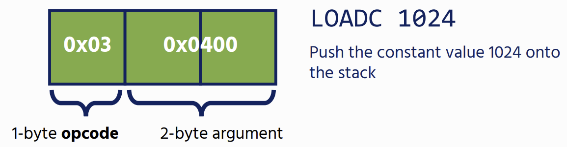
Bytecode
compact representation of program code, suitable for efficient interpretation Instead of storing source code strings, bytecode consists of a 1- byte opcode followed by (optionally) any arguments
they are much faster than treewalk interpreters but compilation to bytecode is easier to implement than native code compilation
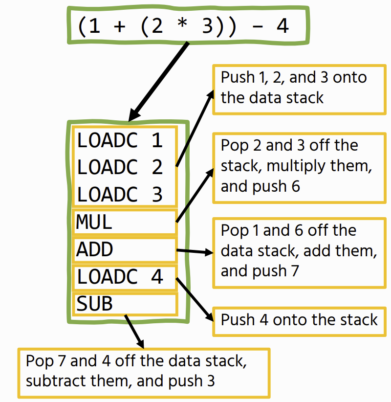
Stack Machines
The basic idea is that we have a stream of instructions that manipulate a data stack
- Operations have a fixed size
SVM
stack-based: instructions use an operand stack rather than having explicit parameters.
Machine State
Code Store
SVM state is a code store containing the machine’s bytecode.
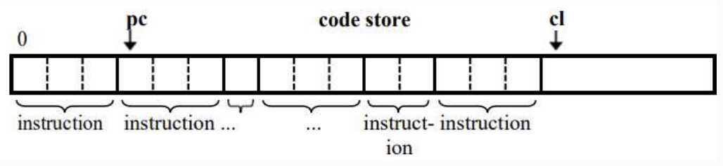
- A program counter (pc) that tracks the current instruction
- A code limit (cl) that marks the end of the code store
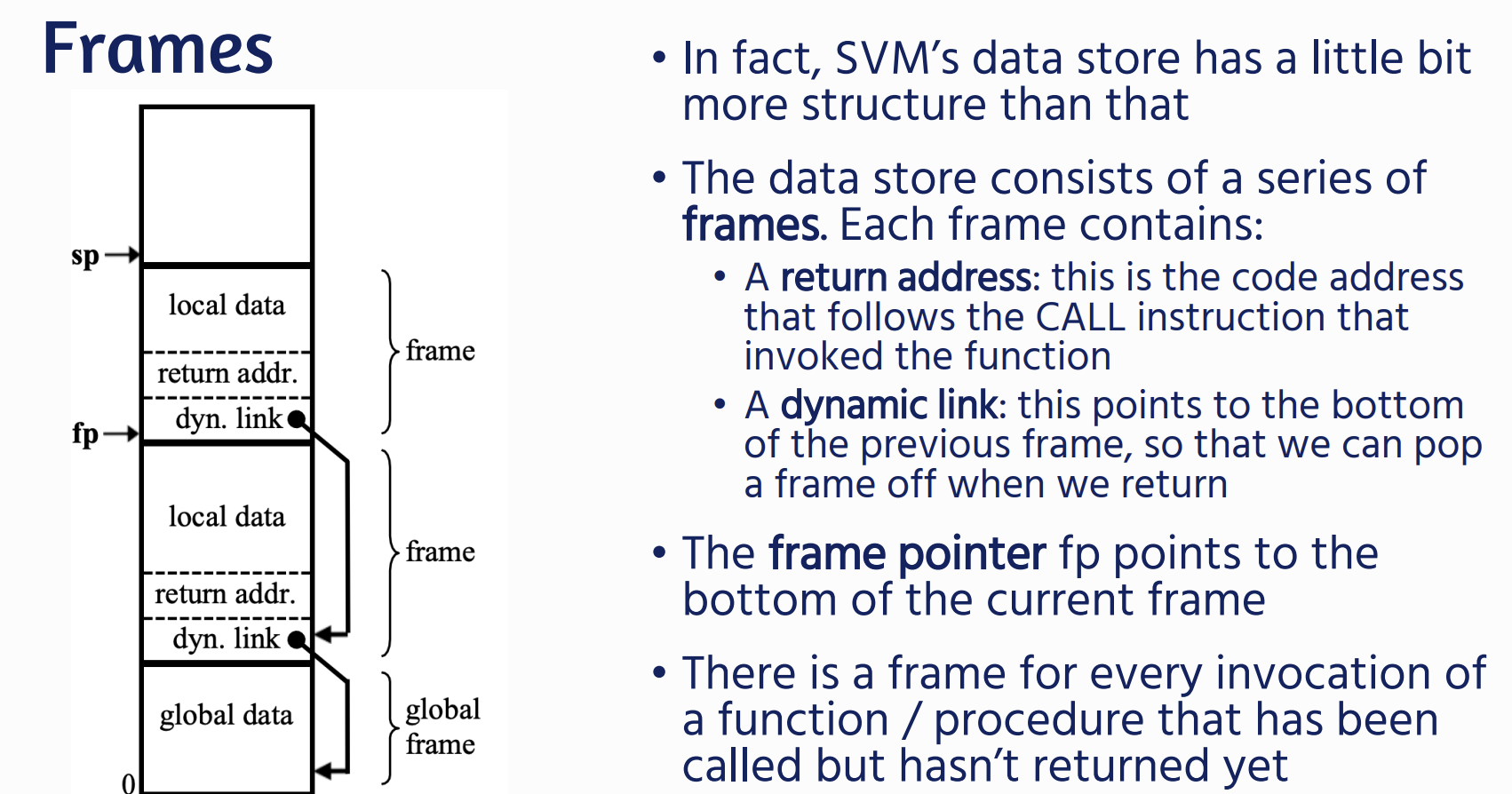
Data Store
| SVM state is a data store containing the program’s data - A stack pointer (sp) that denotes the top of the stack, some data that occurs on the stack, and then global data. - A status register that indicates whether the program is running, halted, or failed. | 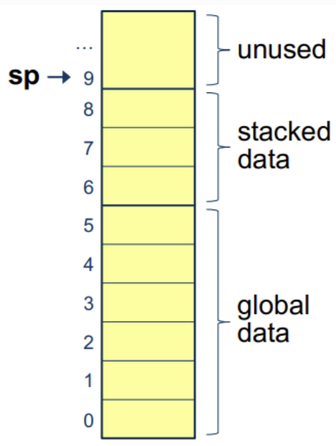 |
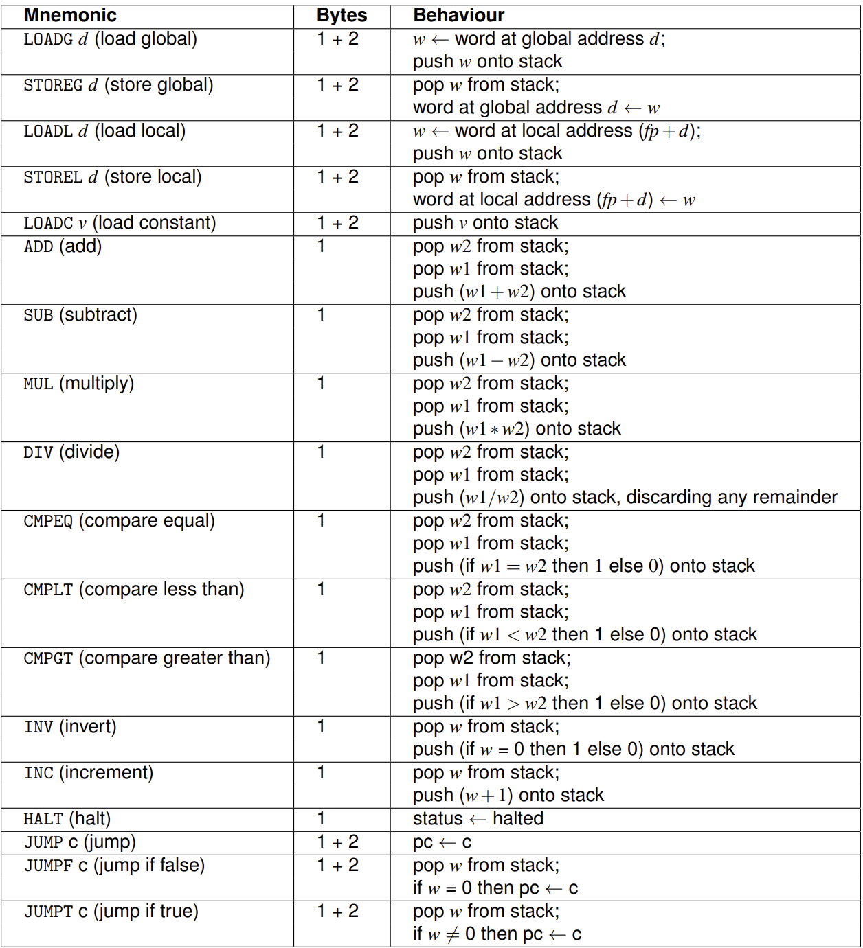
SVM Instructions
Each SVM instruction occupies 1, 2, or 3 bytes:
- Every instruction has a one-byte opcode that identifies the instruction.
- 1-byte instructions do not have any arguments associated with the instruction
- (e.g., instructions such as ADD that only work with the stack)
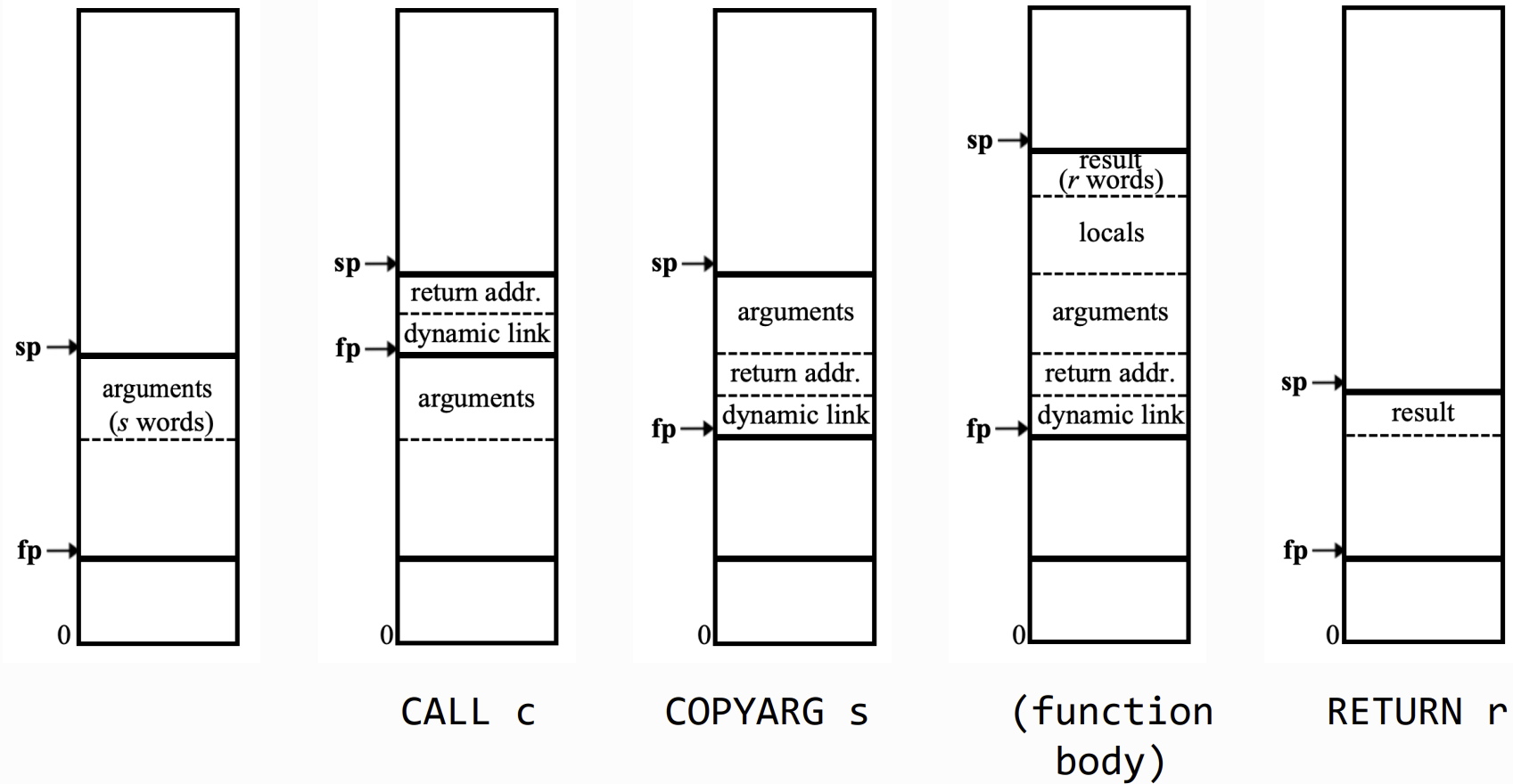
- 2-byte instructions have a (small) argument associated with them
- (e.g., instructions such as RETURN that state the number of words to return)
- 3-byte instructions have an argument associated with them that might need two bytes of storage:
- (e.g., loading a constant onto the stack)
- (e.g., loading a constant onto the stack)
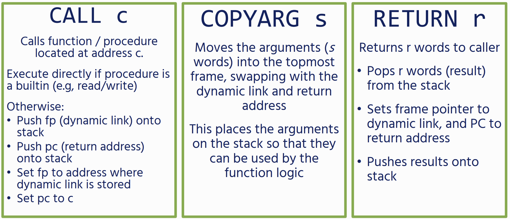
For Functions and Procedures
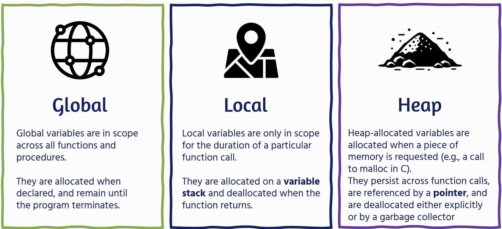
Variables
Whenever we declare a variable, we store its address in an address table Each address is associated with a locale:
- CODE (for function / procedure addresses)
- GLOBAL
- LOCAL
Paradigms
if else
Back-patching
- Emit a placeholder jump
- Remember its position
- Come back later and fill in the correct address
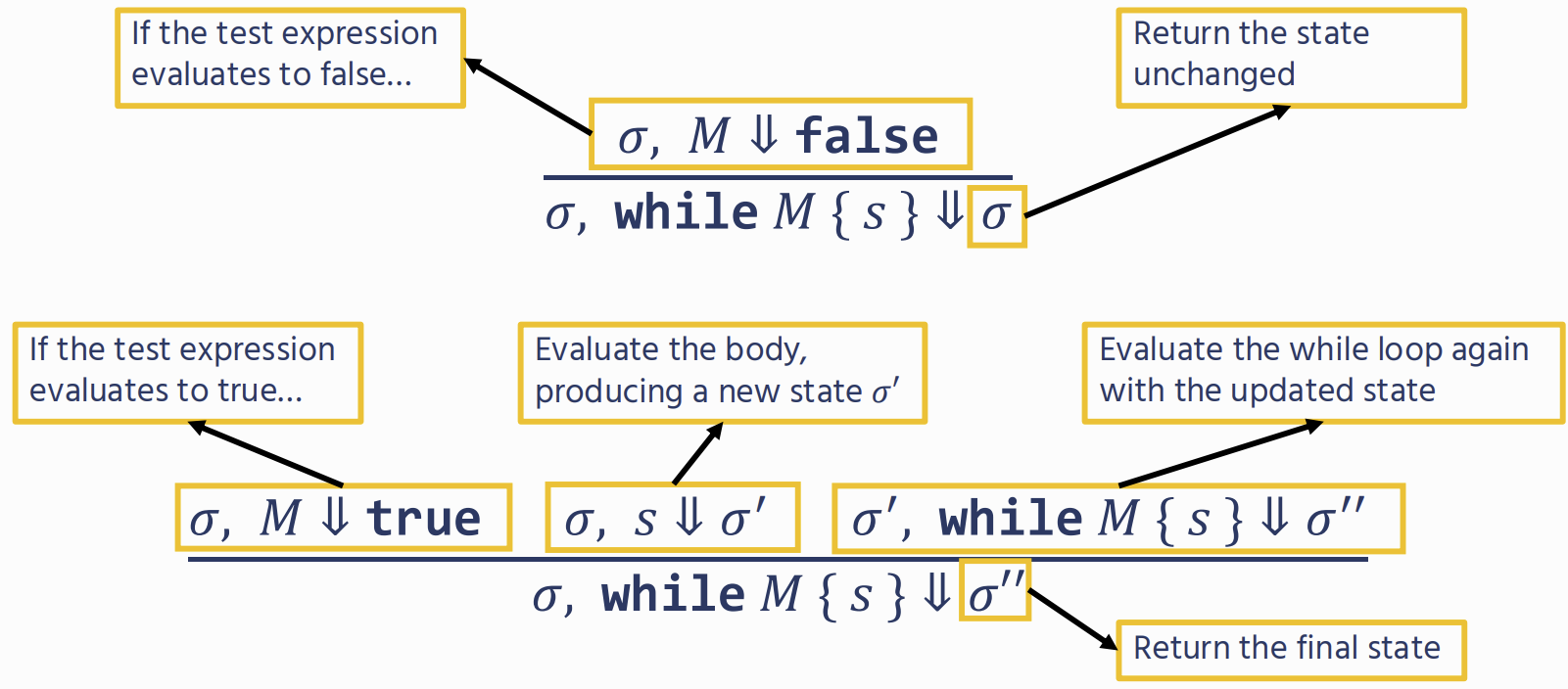
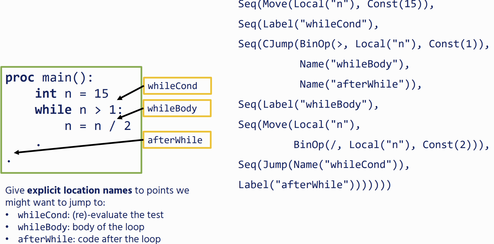
while
- firstly compile the test expression, and emit a JUMPF with a placeholder address
- emit code for the loop body, along with an unconditional jump back to the test
- we back-patch the JUMPF to after the loop body
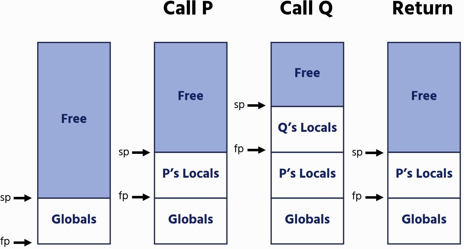
Function and Procedure Calls
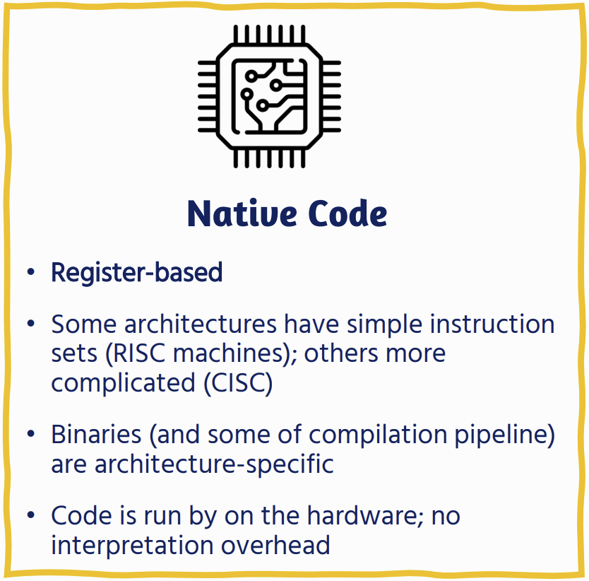
Native Code Generation
 We want to compile natively for:
- Performance: There is no interpretation overhead: code is run directly by the hardware • We can also make use of architecture-specific optimisations
- Bootstrapping: bytecode interpreters need to be written in a compiled language!
- Systems programming: often need to write very low-level code (e.g. that makes use of system calls or inline assembly)
- JIT compilers: can use native-code compilation while interpreting in order to compile based on profiling information
Compilation
Intermediate Representations
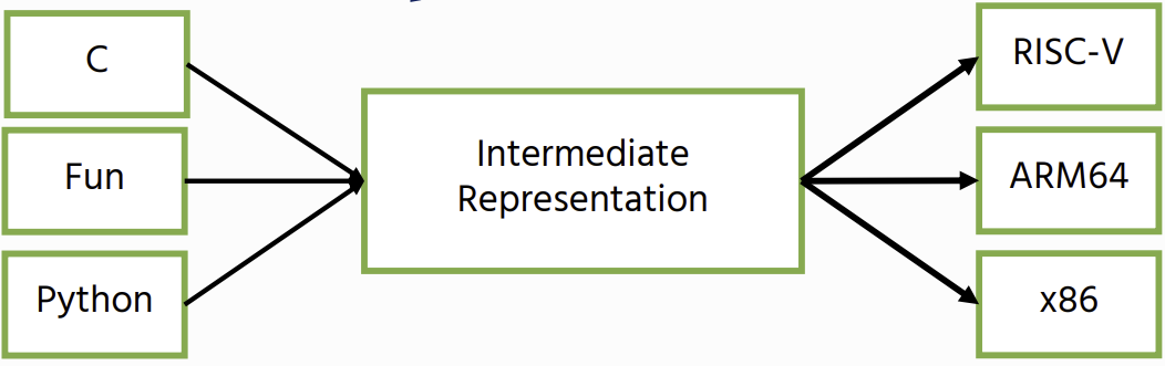 While it is possible to go directly from a program to native code, it is better to compile to an intermediate representation first.
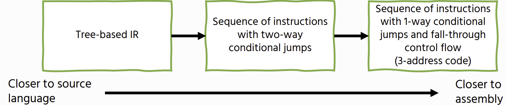
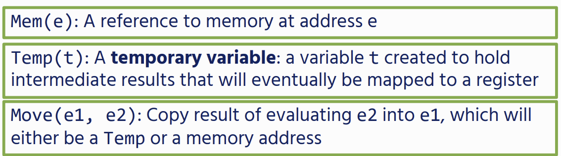
Our IR will form a single tree The IR will contain two entities:
- Expressions: these return a value
- Statements: these perform side-effects labels: these are program locations that we can jump to
Tree based IR
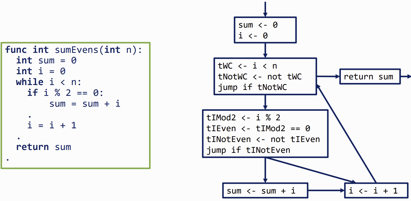
Control-Flow Graphs
Basic Blocks (BB)
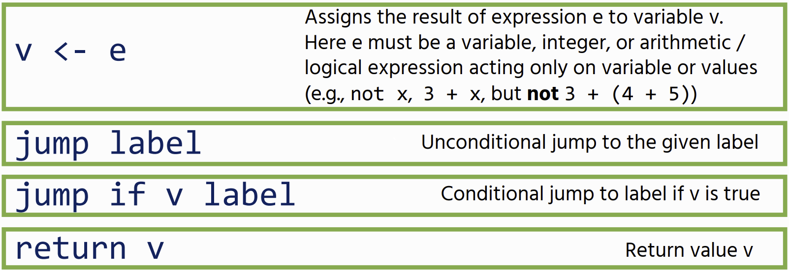
translating a expression into a sequence of instructions
each instruction is a Three-address code
- Each node is a basic block
- Each edge is a jump to another BB (either an explicit, possibly conditional jump, or a fall-through)
- We mark one BB as the entry point, and one as the exit point
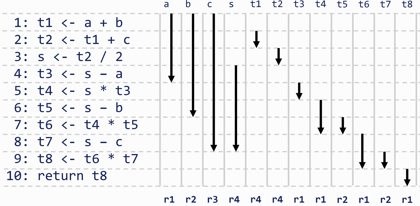
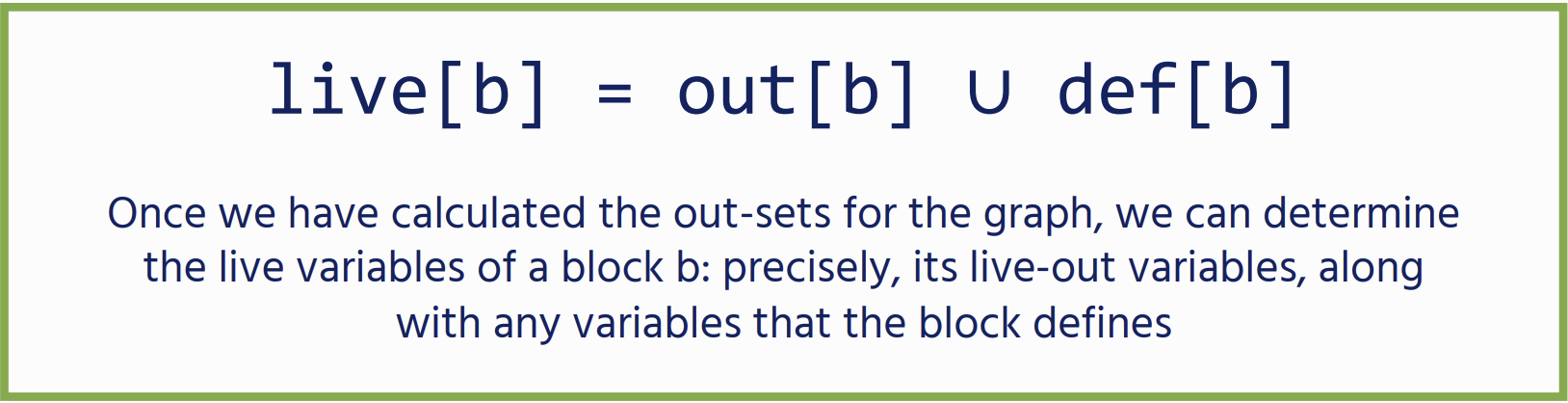
Liveness
gives us the information we can use to allocate variables to physical registers
- to do Liveness analysis we consider a variable live from where it is defined to its final use
Liveness in a Basic Block
the registers required is calculated/allocated based on non-overlapping liveness ranges
Liveness in a Control-Flow Graph
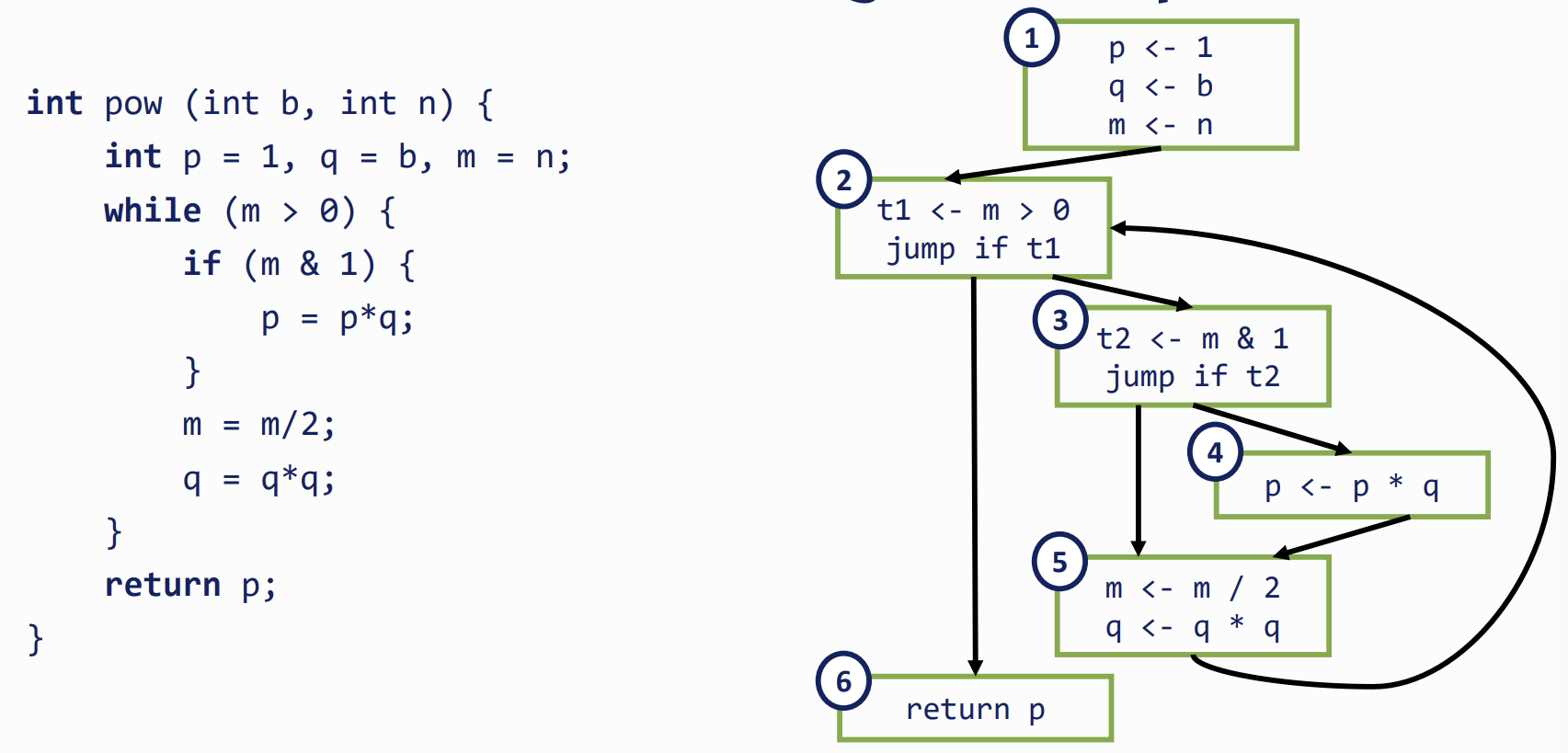
- b and n are only live in BB1
- p is live everywhere (path from assignment both to the return and through the loop)
- m and q are live everywhere except BB6
- t1 is only live in BB2
- t2 is only live in BB3
Definitions
- A node has out-edges that lead to successor nodes: example the out-edges of node 2 are:
- 2 → 3 and 2 → 6 and succ(2) = { 3, 6 }
- A node has in-edges that come from predecessor nodes: example the in-edges of node 5 are:
- 3 → 5 and 4 → 5 and pred(5) = { 3, 4 }
- An assignment to a variable in a node defines that variable: example:
- def(1) = {p, q, m}
- A node uses a variable if it appears on the right-hand side of an assignment: example:
- use(1) = { b, n }
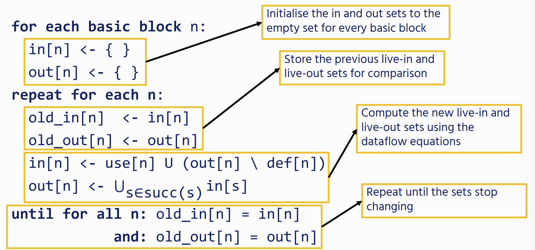
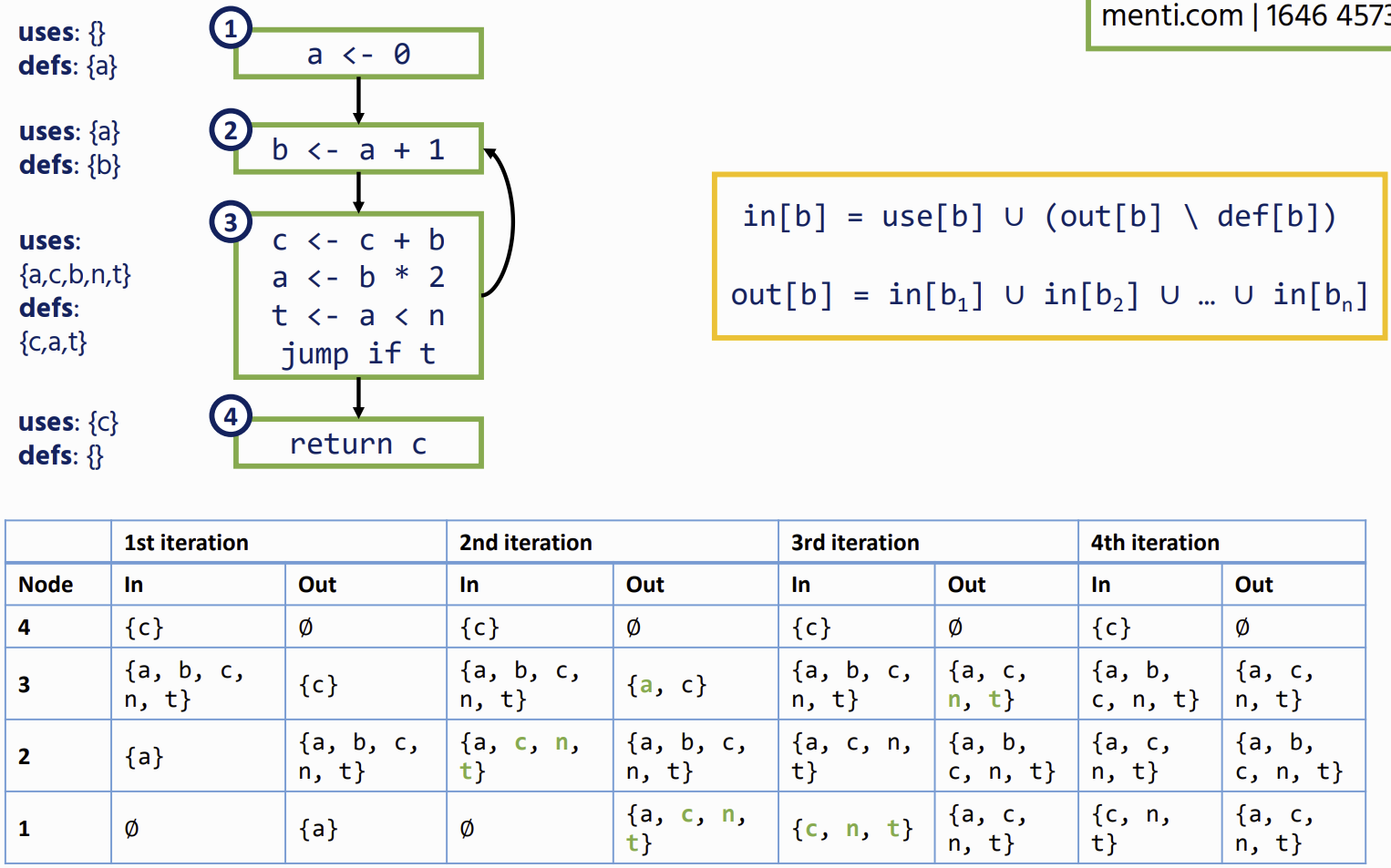
Dataflow Equations
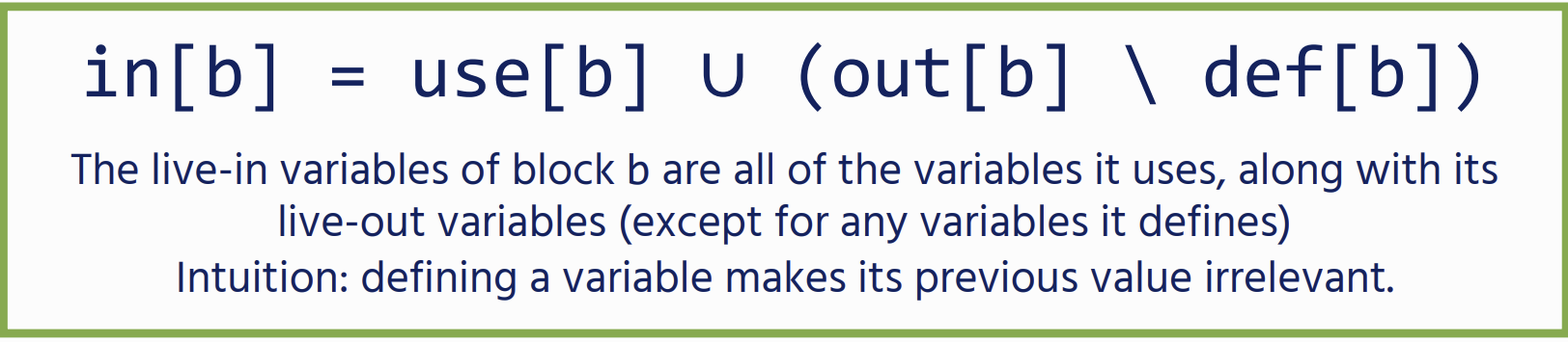
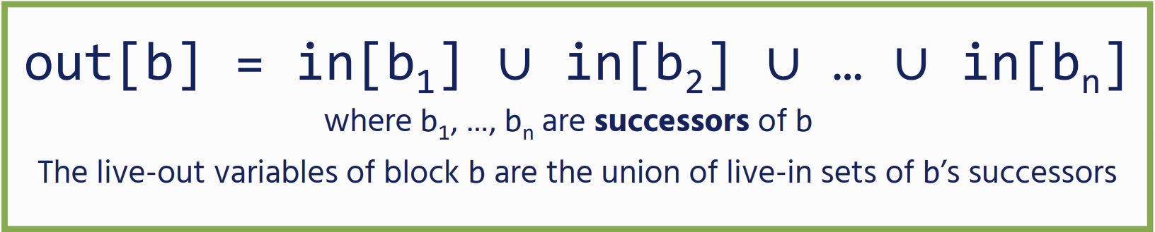
Solving Dataflow Equations
we start from an empty set and iterate the equations, we will eventually arrive at a fixpoint: future iterations will not change the sets
Since we are trying to trace how data flows from its uses to its definitions, it is more efficient to process the CFG backwards
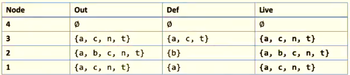
Register Allocation
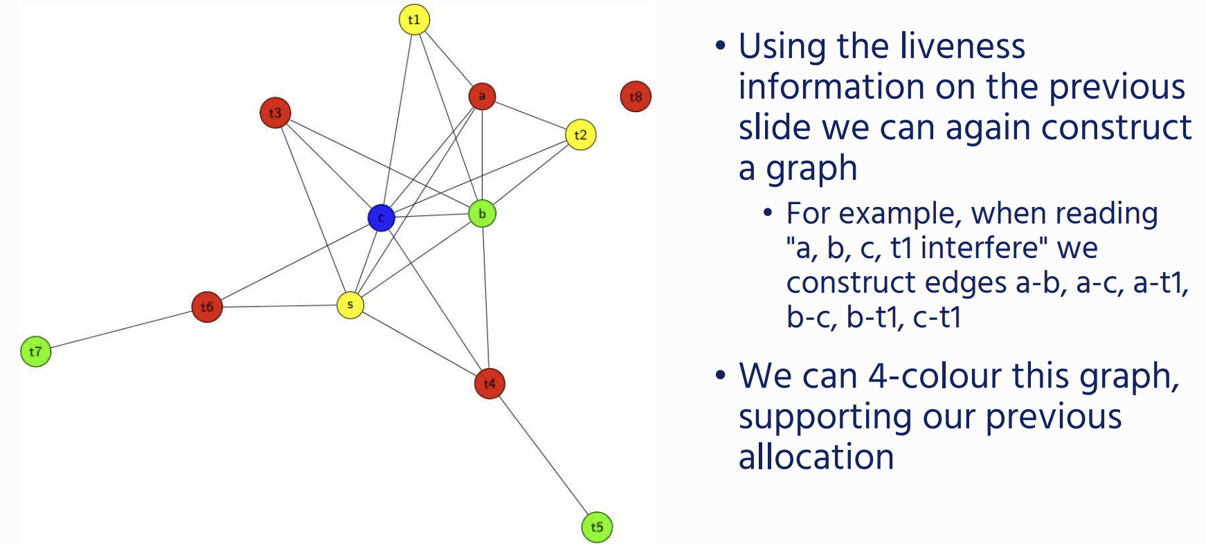
we allocate Register using graph colouring on a interference Graph.
Interference graph
- Every variable is a vertex / node in the graph
- We add an edge between two variables if they are live at the same time (i.e., simultaneously occur in a node’s live-out set).
 Sometimes we will get a graph that we cannot colour with the available number of registers: in this case we will need to write the variable to memory. This is called spilling
Instruction Selection
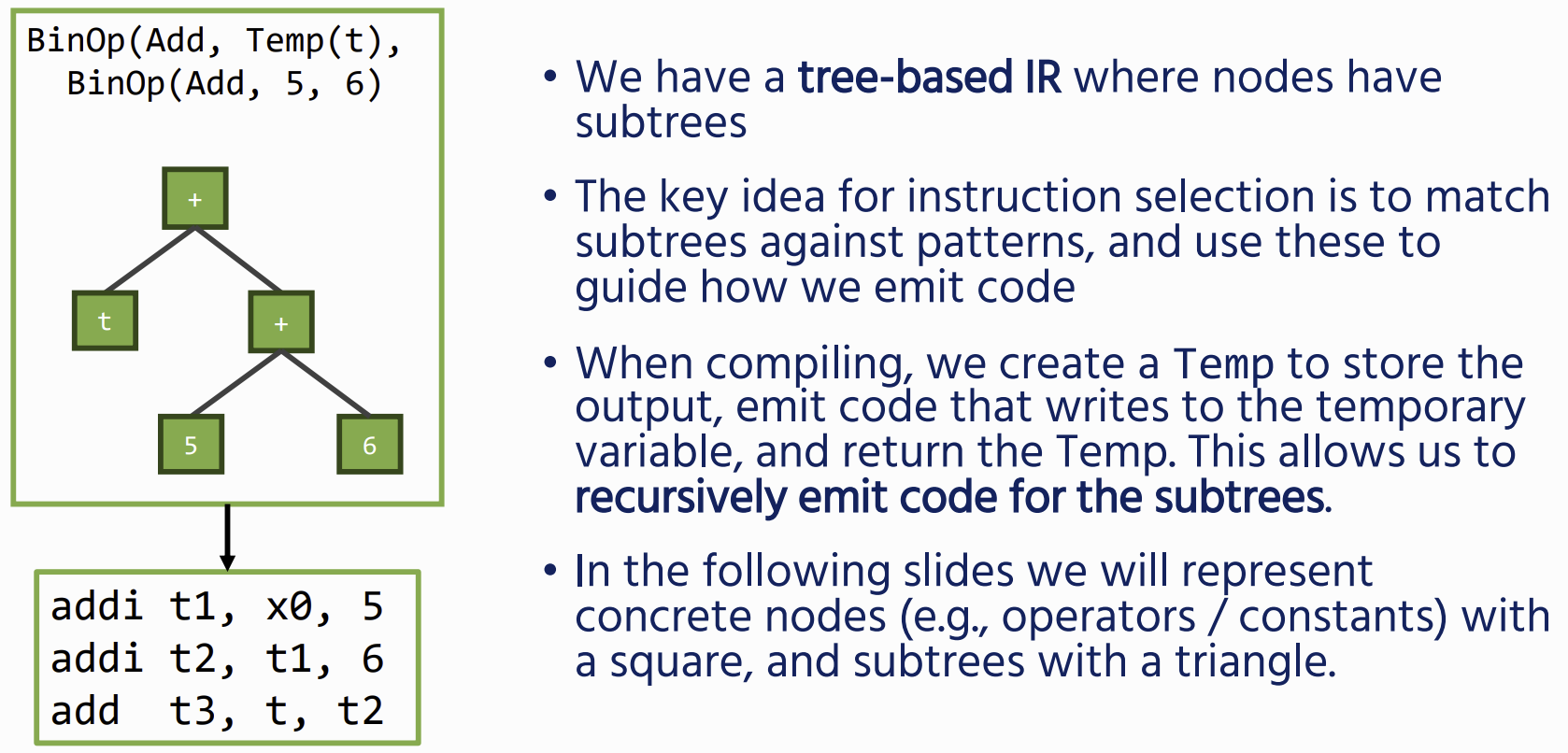 Often there are multiple different ways of compiling the same IR – we ideally want to optimise for, for example the smallest number, or most efficient instructions, this is a job for Instruction selection
Binary Operations
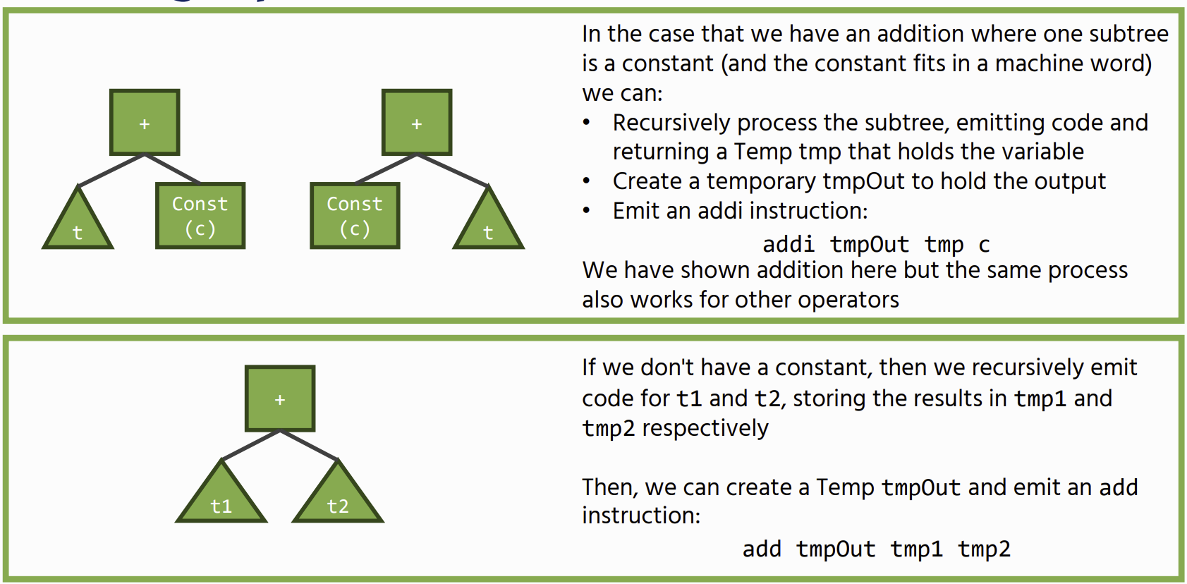
Load Operations
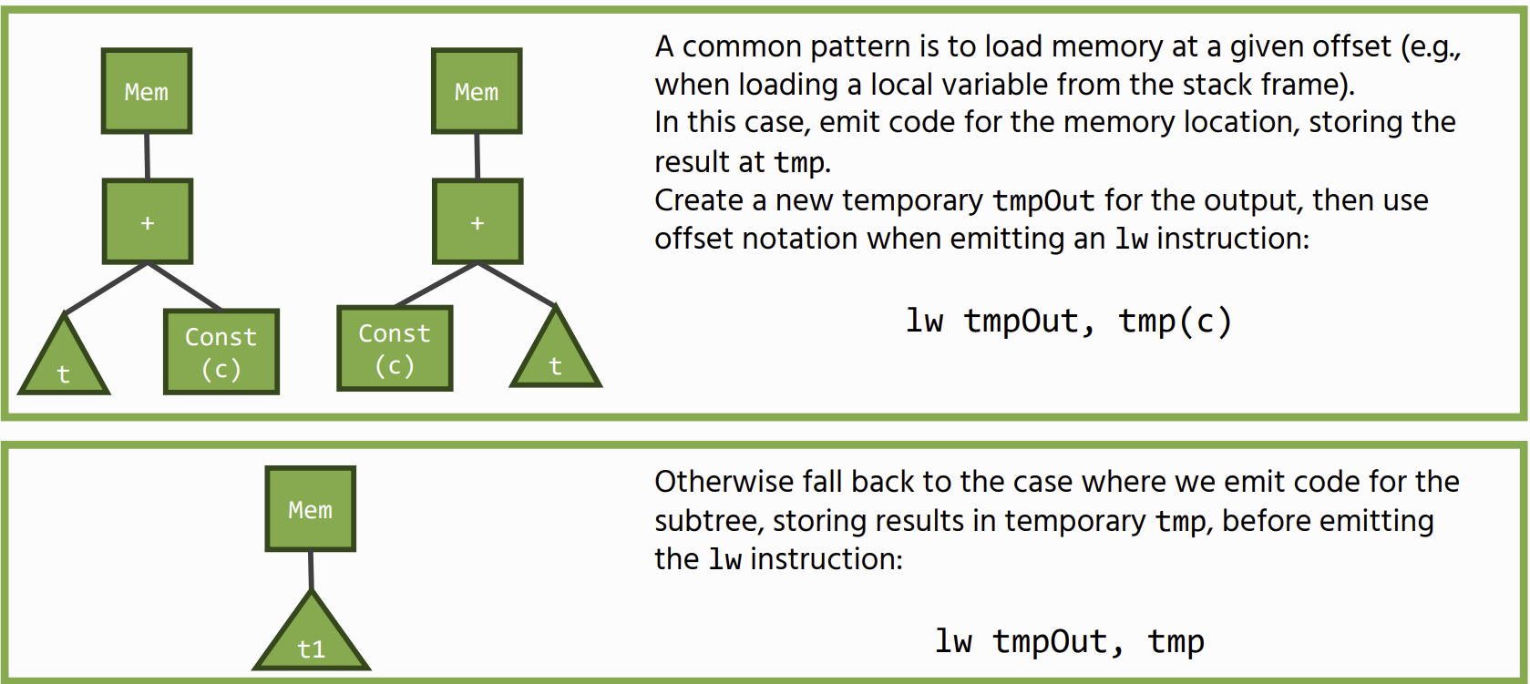 Move statements (stores) follow a similar pattern
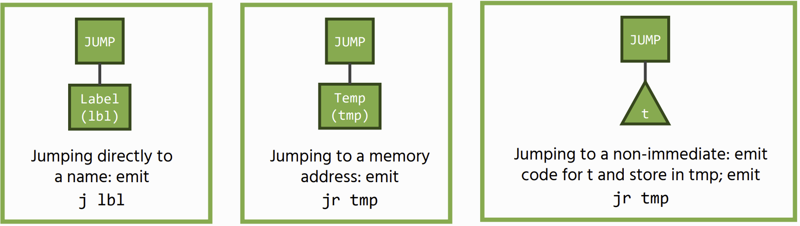
Control Flow: Jumps
There are two types of unconditional jumps: a direct jump to a name, or an indirect jump to the address contained in a register
 Conditional jumps are similar: we match on the binary operator and generate the corresponding branch instruction
Instruction Selection Algorithm: Maximal Munch
Say we have some IR tree t and a set of instruction patterns ps. To cover t using ps:
maximalMunch(t, ps):
	p = largest pattern in ps that covers the top of t
	uncoveredSubtrees = subtrees of t not covered by p
	for s in uncoveredSubtrees:
		maximalMunch(s, ps)
	emit(t, p) // emit code for pattern p
The algorithm is linear in the size of t and produces a minimal number of instructions for the given pattern set